


CGL (C Graphics Lib)
In this homework, the goal was to implement a simple rasterizer with features such as drawing triangles, supersampling, hierarchal transforms, and texture mapping with antialiasing, resulting in a functional vector graphics renderer. I learnt quite a bit about each of the sampling algorithms and texture mapping algorithms implemented throughout the project. I also learnt more about the sampling pipeline and how to represent the abstractions of sample buffer, pixels, texels, and coordinate systems through the data structures used in this project.
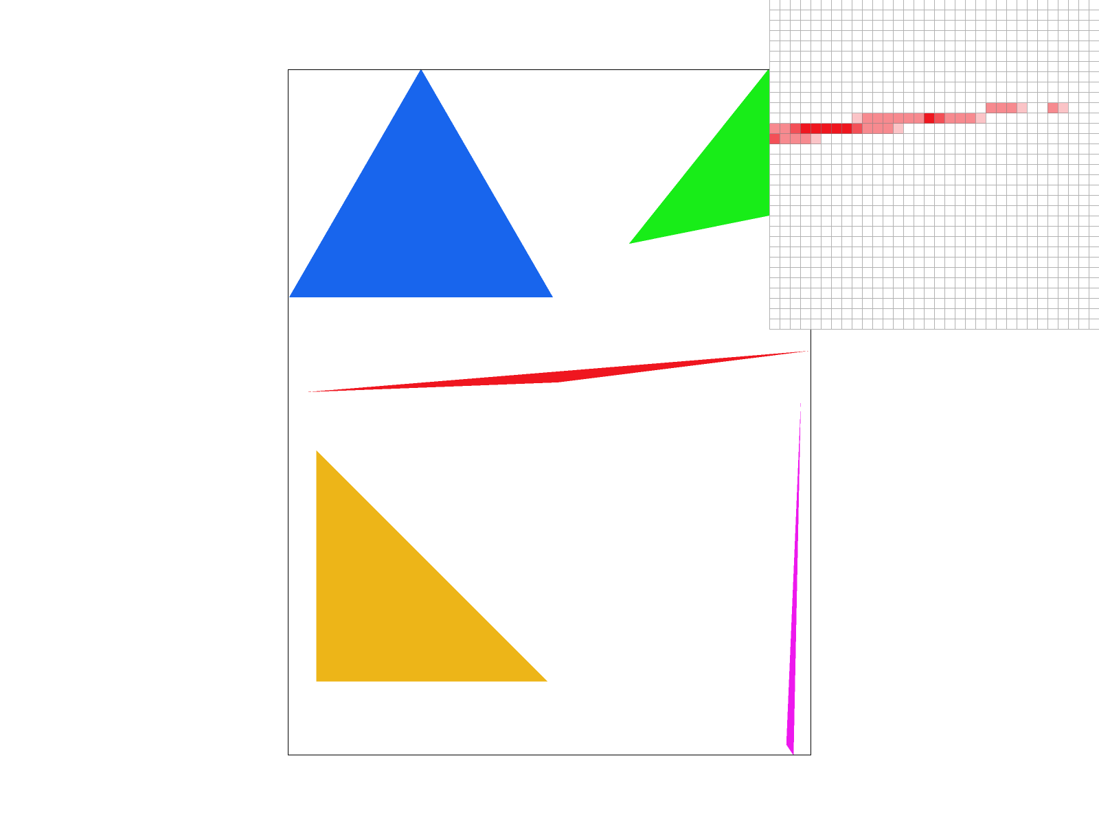
In order to rasterize triangles to the frame buffer, I check if the center of each pixel is within the triangle.
The rasterize_triangle function takes in coordinates for each of the three corners of the triangle.
My implementation first determines what the smallest bounding box (calculated by determining the lowest and
highest x and y values that the triangle covered) around the triangle. Then, it iterates through each pixel in
the bounding box and checks if the center of the pixel is within the triangle. We check if the center of the
pixel (x + 0.5, y + 0.5) is in the triangle by checking to see that it is within the three edges of
the triangle. If it is, the pixel is filled in with the color of the triangle. This handles coordinates received
in the clockwise direction, but to include coordinates in the counter-clockwise direction, I reversed the
inequality check.
This algorithm is no worse than traversing each sample individually in the bounding box of the triangle and determining if it's in the triangle because we still iterate through all the points in the bounding box. There is no optimization or short circuiting that reduces the number of pixels traversed.
In this task, I implemented supersampling by updating the sample_buffer data structure and modifying
certain algorithms. Supersampling is useful because it allows us to antialias and reduce the jaggies in our
images, making pixels seem smoother zoomed out. The modifications I made to the rasterization pipeline was to
first change the size of the sample_buffer to include the number of samples we wanted to sample,
width * height * sample_rate. Now, each (x, y) pixel will be represented by a
sample_rate number of samples that will be averaged in order to downsample to determine the color of the
original pixel. I added a new fill_sample function which fills in the color of a specific sample
for an (x, y) pixel and updates its color in the sample_buffer by using a new indexing method:
sample_buffer[sample_rate * (y * width + x) + s]. I updated the fill_pixel sample to
stay consistent for points and lines by calling fill_sample for the number of samples in the pixel,
effectively making sure that all samples have the same color. In rasterize_triangle, I now iterated
through each sample, rather than pixel to check if we were within bounds, and called fill_sample
instead of fill_pixel. Finally, in resolve_to_framebuffer, I updated the frame buffer
by getting all samples that corresponded to an (x, y) pixel and averaging the RGB values of all the
samples to get the final color, which was then resolved to the framebuffer target.


Sample rates of 1, 4, 9, and 16
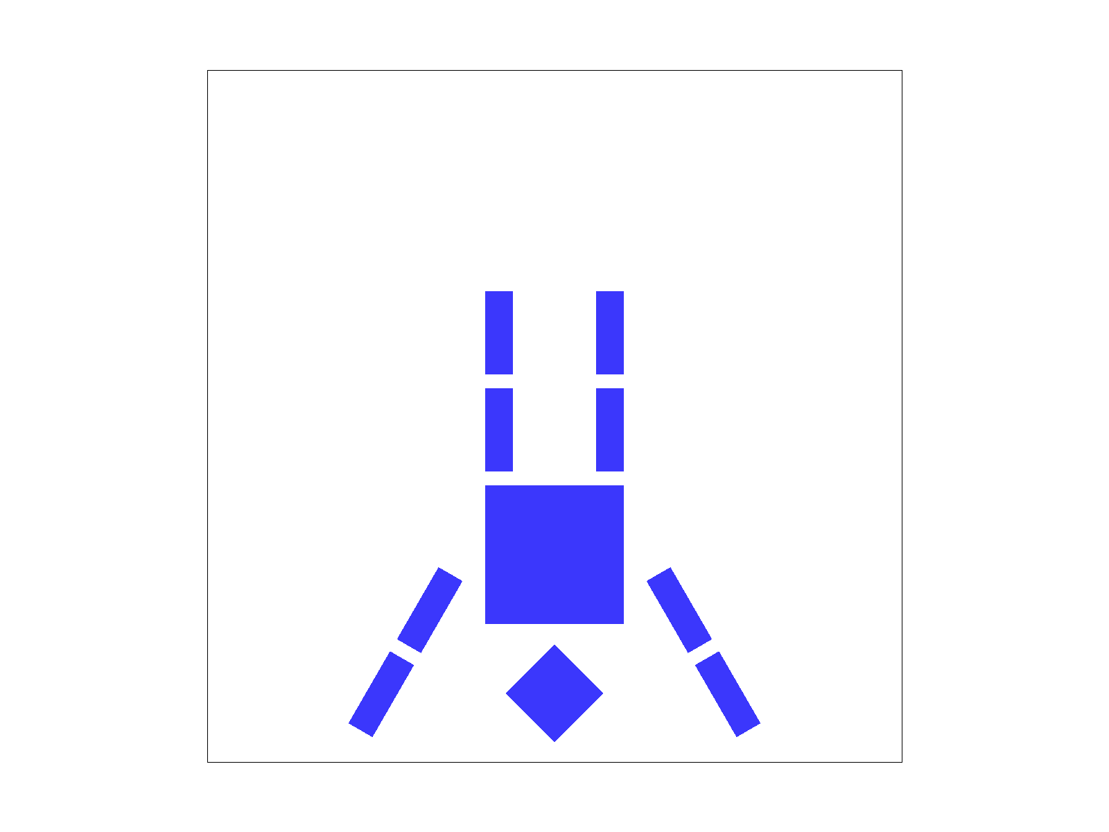
Cubeman stands on their head
Barycentric coordinates work by determining our color based on the distance each point is from each vertex. As we can see with our triangle, each vertex is red, green, or blue. We end up with a gradient triangle as our final image because for each point not at the vertices, we calculate a certain weight of red, green, and blue based on distance and end up with a weighted sum of RGB colors within the triangle.
We calculate the barycentric coordinates by solving for the value of each our new color coordinate system
(alpha, beta, and gamma) based on the current (x, y)
coordinate. This allows us to assign colors based on the strength of how close each of the points are too the .
We then calculate the color by interpolating across the colors passed in to the function to get a weighted sum:
alpha * c0 + beta * c1 + gamma * c2. This is our new value for the color at the point
(x, y) so we call fill_sample with the new color.
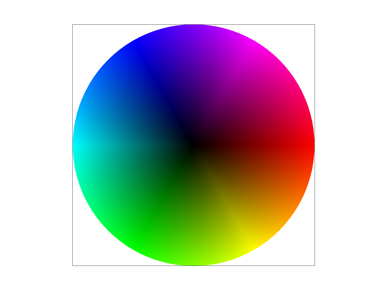
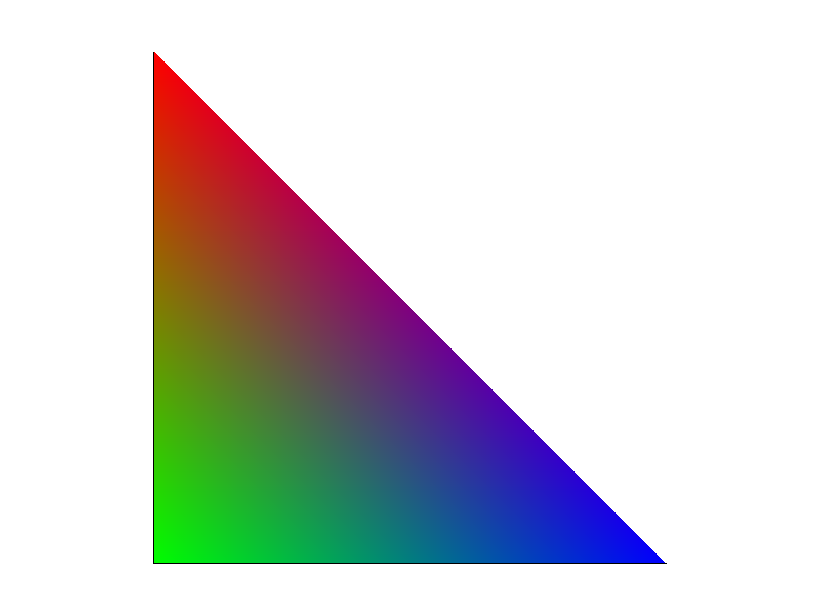
Barycentric circle and triangle
With texture mapping, the goal is to interpolate to find the texture coordinate (u, v) for each
(x, y) coordinate. We can do this using nearest and bilinear sampling methods.
I implemented texture mapping by calculating the uv coordinates based on the barycentric coordinates
that had been calculated. I initialized the SampleParams struct with the uv values and
then sampled from the texture based on which sampling method we wanted to use. The sample function
returns a color which can then be used to fill the sample.
In the sample_nearest function, I found the nearest pixel to our uv coordinate and then
returned the color of that pixel on the mipmap. To implement sample_bilinear, I got the nearest 4
texels to our uv coordinate. After, getting the colors, I linearly interpolated in both directions
and then did a final interpolation of the two interpolations to get the final color value.


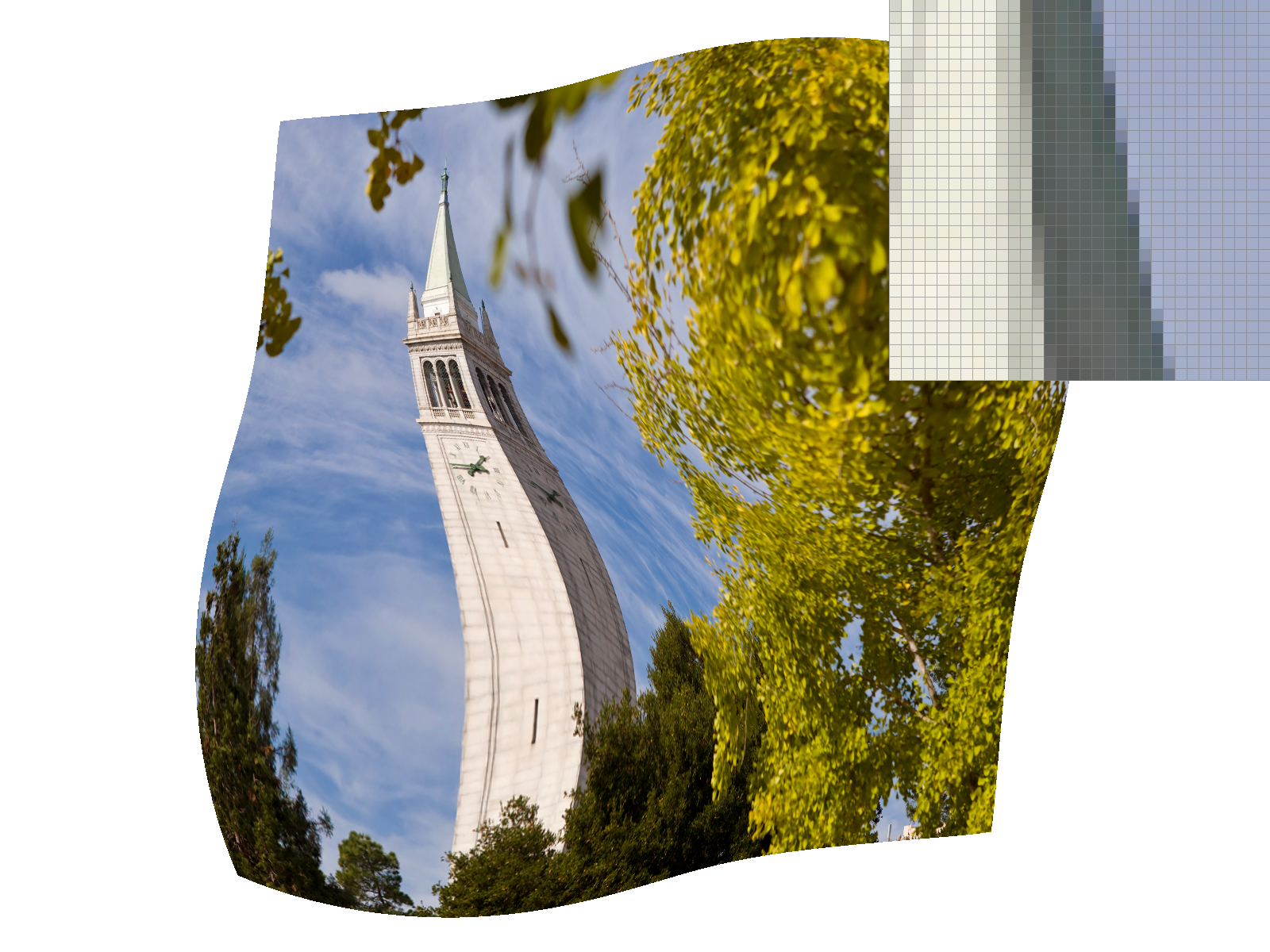
Nearest with sample_rate 1 and 16
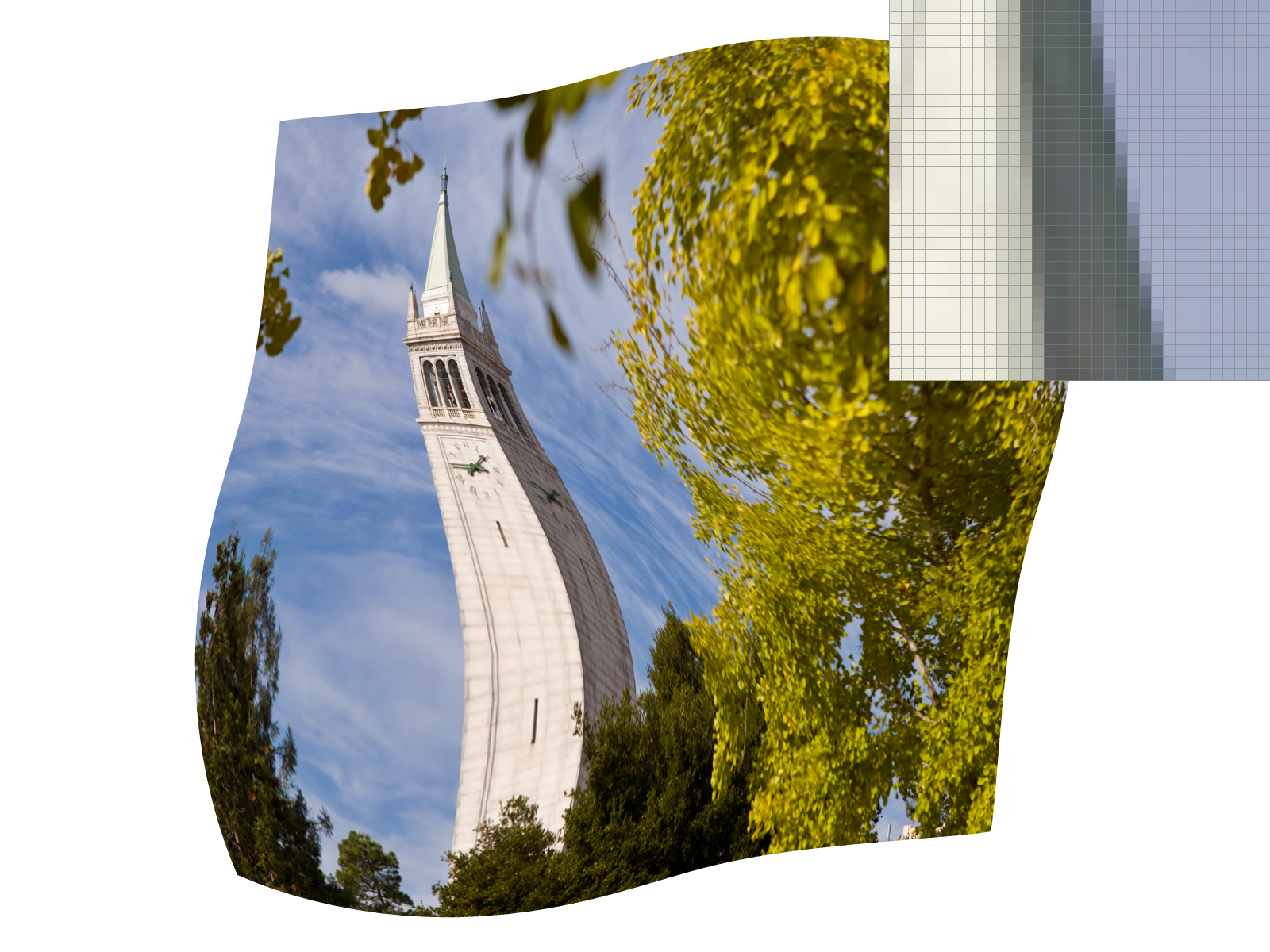
Bilinear with sample_rate 1 and 16
Based on these images, a higher sampling rate helps create a blurring effect that reduces jaggies no matter which sampling method is used for texture mapping. Bilinear seems to be better at blending nearby texels as we zoom in and creates the illusion of straight lines even without a higher sampling rate. Combining both bilinear sampling and high sampling rate allows us to get smooth and clear details even when zoomed in quite a bit. The tradeoffs are that bilinear sampling takes more time to render. If we have an image with lots of finer detail, bilinear sampling will be able to preserve these details much more than nearest sampling.
In level sampling, we add the calculation of samples that represent the downsampled image that we can use to
improve the resolution and pick better texture samples that correspond with the amount of aliasing occuring.The
modifications in the calculation include calculating derivatives that quantify the difference between texture
coordinates that are near each other. In order to make these changes smoother, I used linear interpolation again
to smooth out the shifts between mipmap levels. The sample function is modified to allow for both
pixel sampling and level sampling to get trilinear texture filtering.
Now that the sampling technique can be modified using pixel sampling, level sampling, and
sample_rate, I've found that the pixel sampling and level sampling take longer to render than
changes to sample_rate. Antialiasing seems better with level sampling and supersampling. I think
level sampling and pixel sampling work better when we are aiming to have our textures be smoother as we zoom in.
Zooming in is definitely the greatest memory usage and speed in terms of having the ability to render everything
at a specific framerate.


[L_ZERO and P_NEAREST] and [L_ZERO and P_LINEAR]

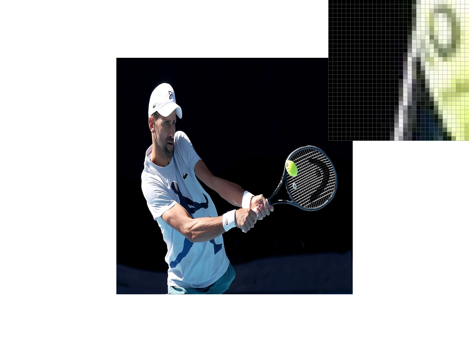
[L_NEAREST and P_NEAREST] and [L_NEAREST and P_LINEAR]
In this homework, the goal was to implement a geometric modeling techniques. I was able to implement the topics we had learnt in class including Bezier curves and practice half edge mesh representations throughout this homework. The most interesting part (and challenging) was understanding and correctly using the half edge mesh representation. I found that drawing images of before and after and writing out the pointers before coding to be helpful for this. I've had previous experience doing modeling in Maya so it was really cool to see the math and look at what happens to each triangle when you add subdivisions or box model.
De Casteljau's algorithm works by using recursive linear interpolation to evaluate points on Bezier curves.
Linear interpolation works by computing the control points at the previous level, based on t. Given
an original n points, we evaluate n - 1 points to get a new set of points. We
recursively repeat this until we get a final point.
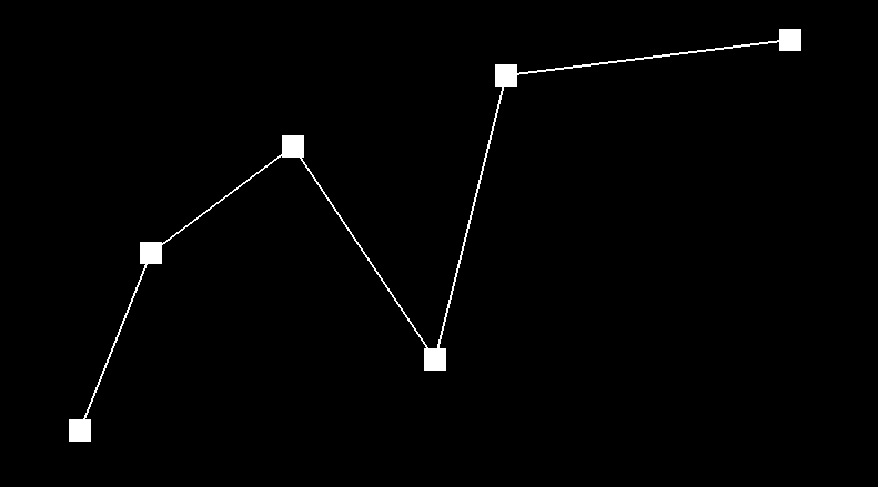
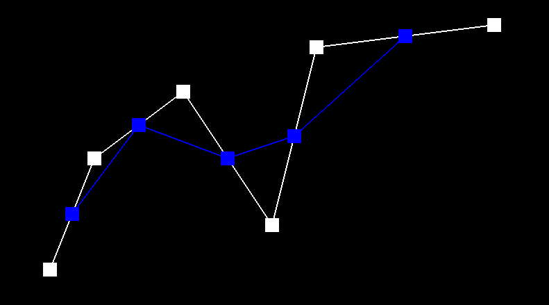
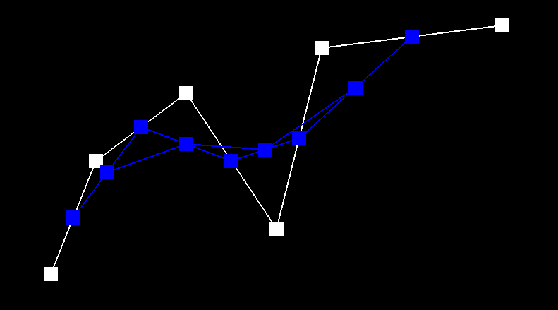
step 1, step 2, step 3

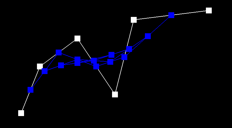
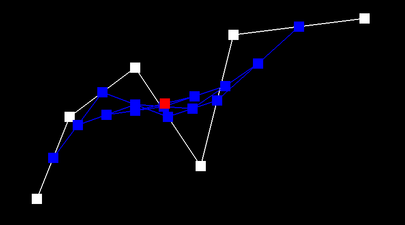
step 3, step 4, step 5
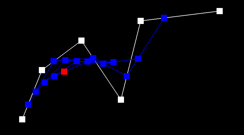
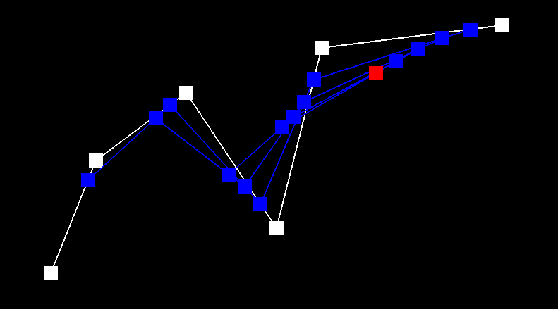
modifying parameter t
First, I extend de Casteljau to Bezier surfaces by first calculating the evaluateStep on 3D points
instead of 2D points. I then implemented the evaluate1D function by recursively calling
evaluateStep for all n points and returning the final point. Finally, the evaluate
function first evaluates n vectors using u as our parameter for t. Then,
I evaluate these vectors in another axis using v as our parameter, which returns our final point.
Ultimately, we extend to one more dimension to compute Bezier surfaces.
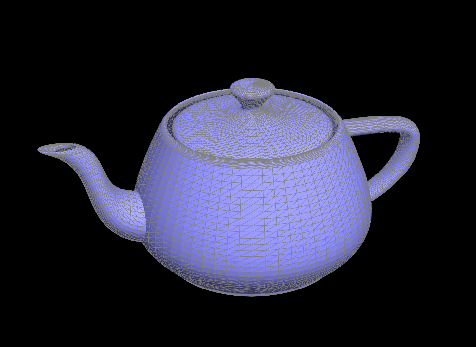
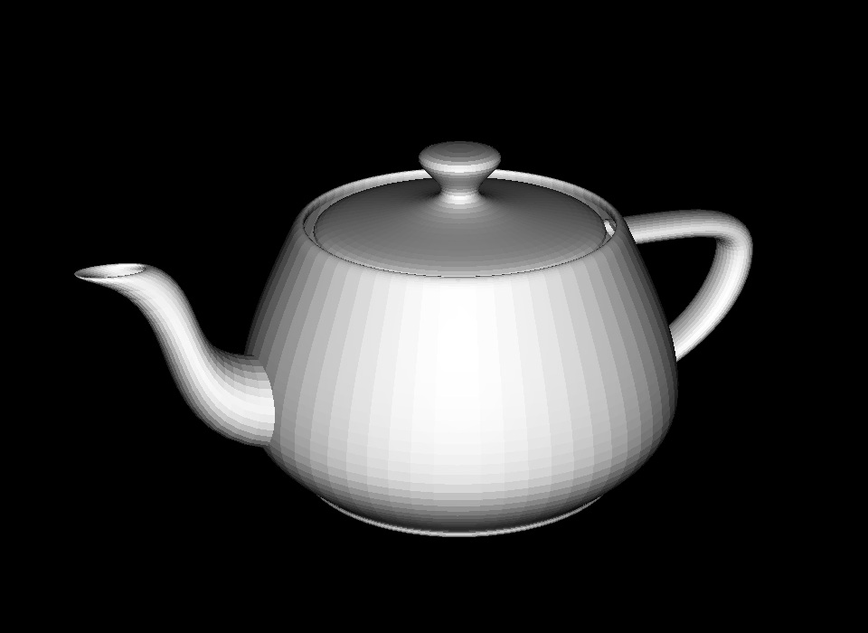
🫖 teapot!
In order have cleaner Phong shading, we calculate area-weighted vertex normals for each face. In order to do this, I first found all vertices for a specific face. To find the normal vector to this face, I took the cross product of two perpendicular vectors and made sure that the normal was pointing outwards. Finally, I summed all the normals across all of the faces and returned the normalized output. Since I'm not modifying any halfedges, I also made sure to use HalfEdgeCIter.
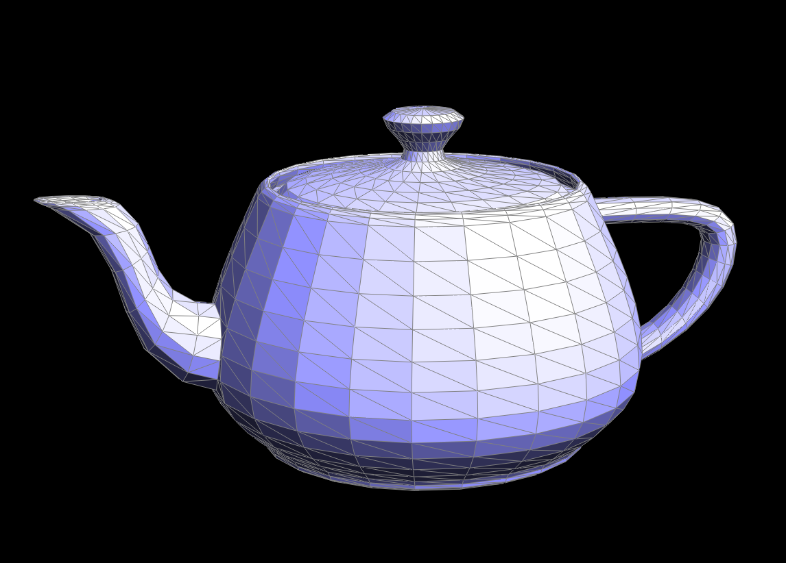
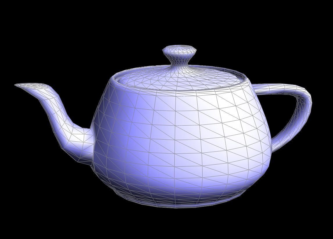
flat shading / phong shading using normals
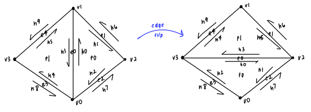
In order to implement the edge flip algorithm, I first drew out this picture above and then wrote out all the pointers that changed throughout the flip and updated them accordingly in the code. Since edge flip doesn't require adding elements or deleting them, I found the implementation pretty straightforward and didn't face any bugs. I realized after completing this that a few operations and assignments could be simplified and accordinly updated that in my edge split implementation.
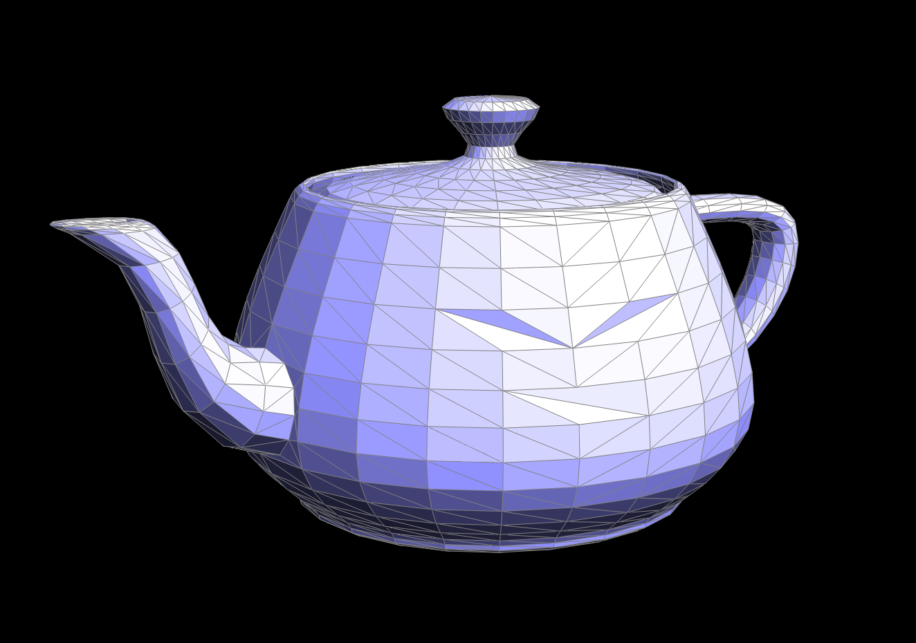
To implement, edge split I followed similar steps as edge flip but also added in a new vertex, two additional faces, and new halfedges and edges. I found the setNeighborsfunction to be quite useful here in order to update all of the pointers of one halfedge at once. Initially, I found no issues with my edge split function but when completing upsampling (below) I realized that a few halfedges were being modified incorrectly which allowed me to fix my implementation. I also added support for labeling the new vertices and edges with isNew = true in the edge split function so that when I edge split in unsample method only the new edges will be flipped.
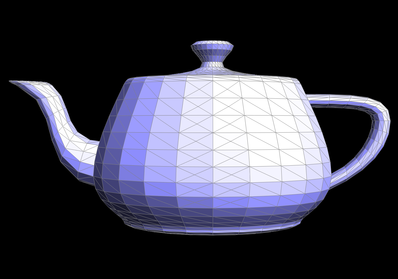

edge split / edge split and flip
I implemented loop subdivision by following the guidelines in the code. I started off by calculating and saving the new positions of the vertices to be updated in the future, using the equation (1 - n * u) * v-{'>'}position + u * neighborPositionSum. I then computed the vertex position of a current edge using the values of the vertices sharing an edge and the equation (3.0 / 8.0) * (A-{'>'}position + B-{'>'}position) + (1.0 / 8.0) * (C-{'>'}position + D-{'>'}position). I also saved a list of originalEdges during this process so that I could split only the mesh edges that were from the original mesh in order to not run in an infinite loop. Here, I updated my edgeSplit function to mark new edges as new so that I wouldn't overflip edges. I then flipped edges based on whether it was connecting an old and new vertex and if it was a new edge. Finally, I updated the position of all the vertices.
As we can see below, the mesh looks nothing like a cube as we increase subdivisions. We achieve a more spherical shape over time but not truly spherical as it maintains part of its squareness.
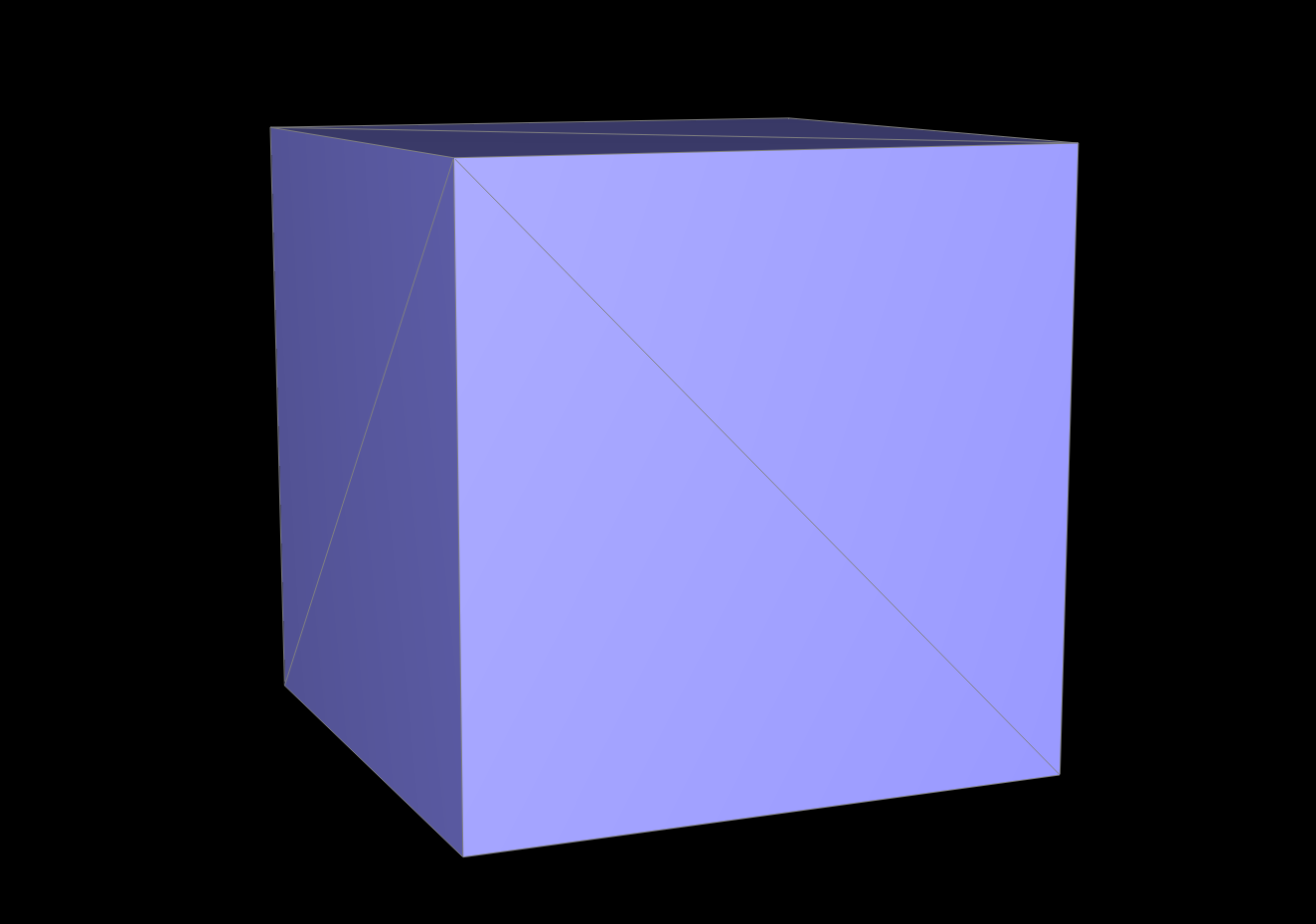
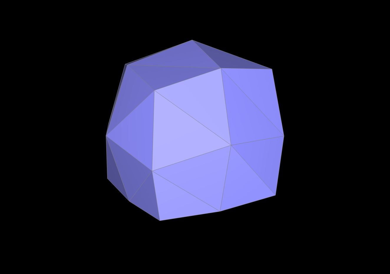
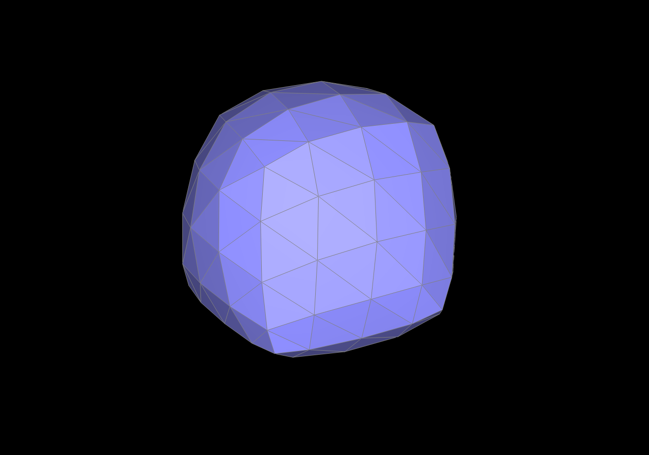
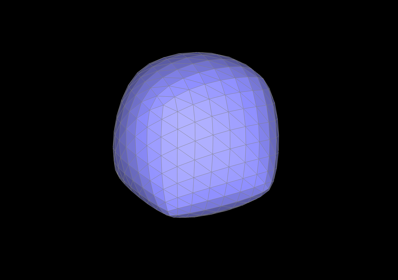
level 0 / level 1 / level 2 / level 3
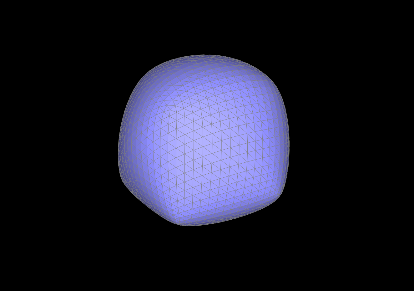
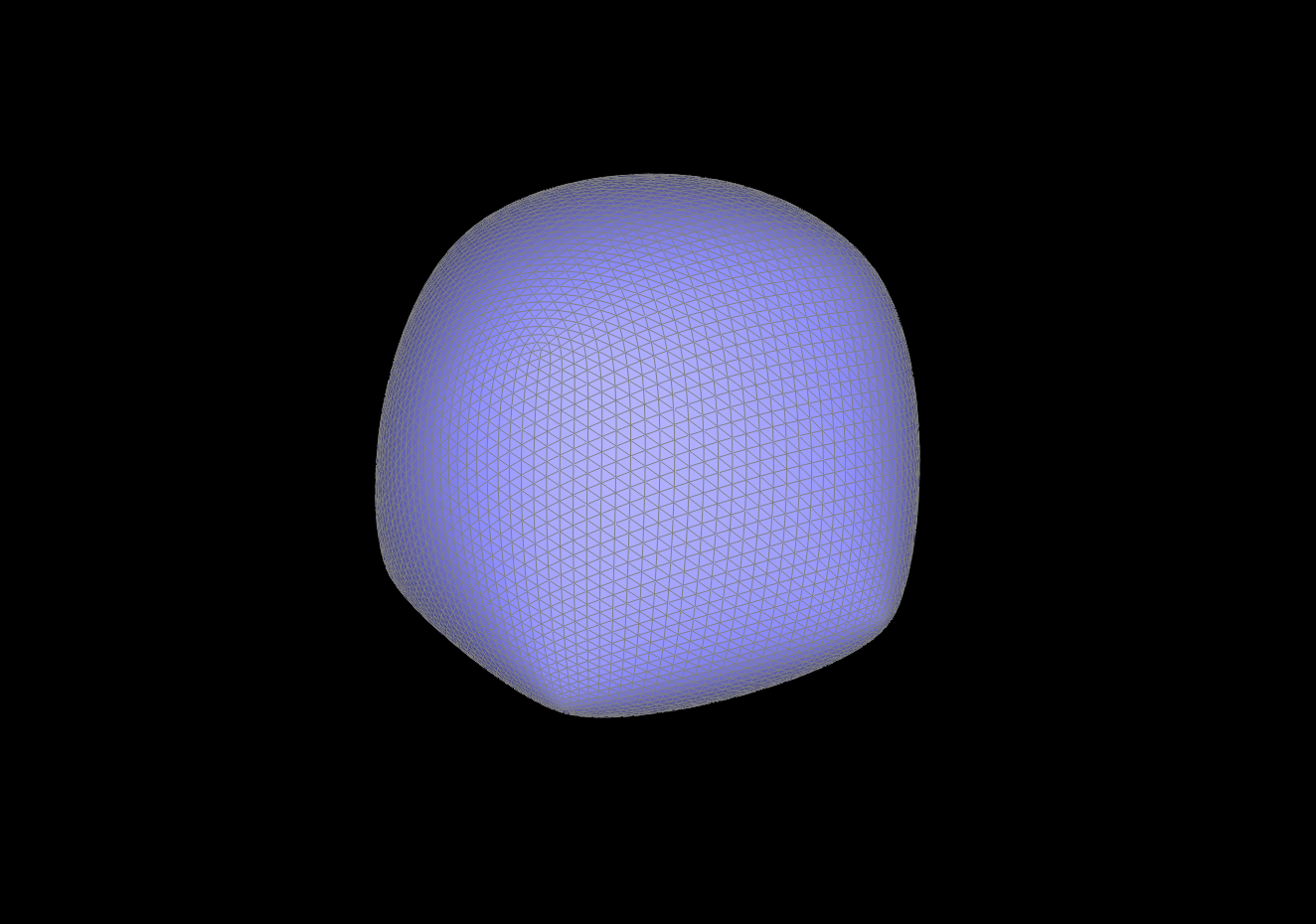
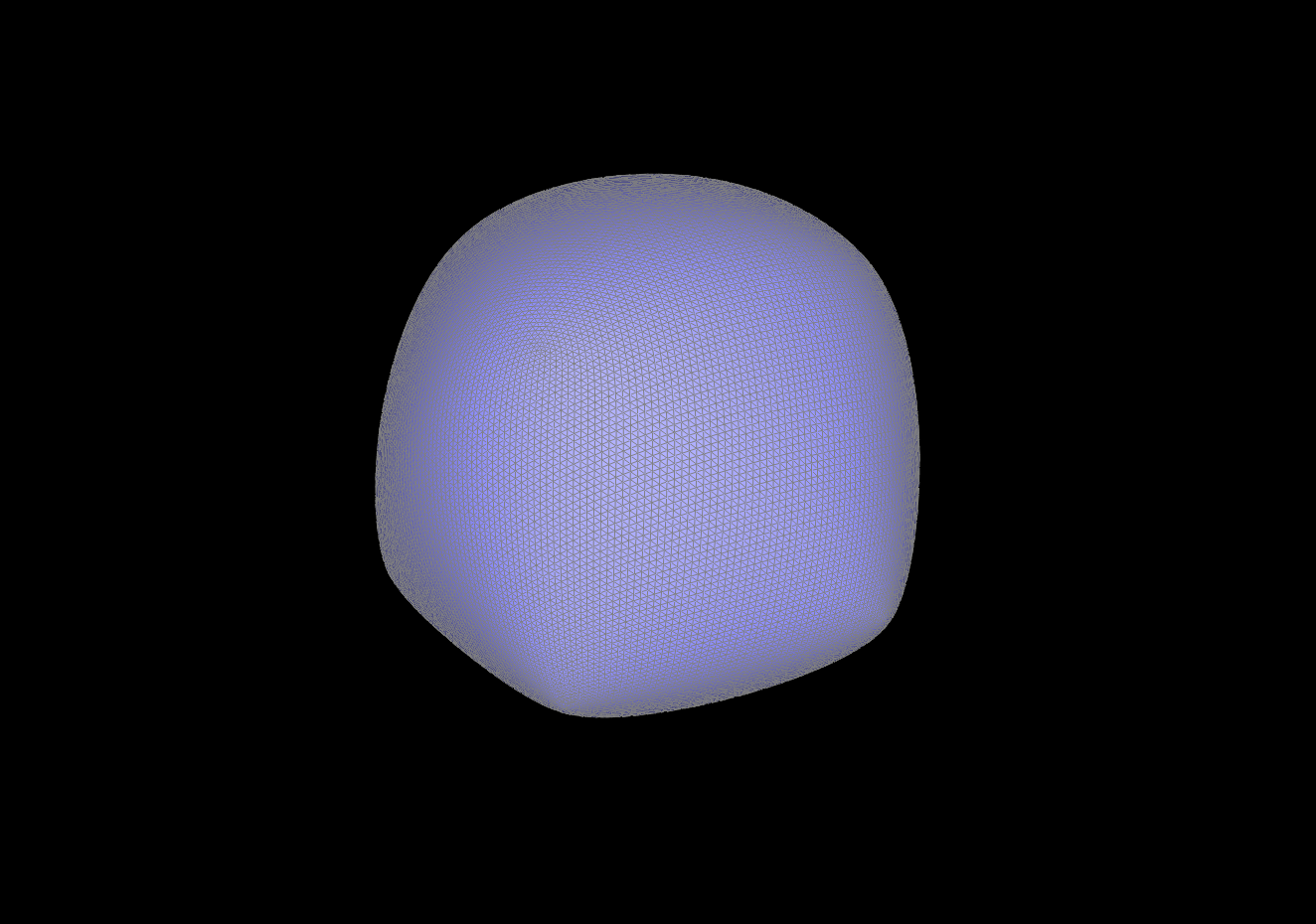
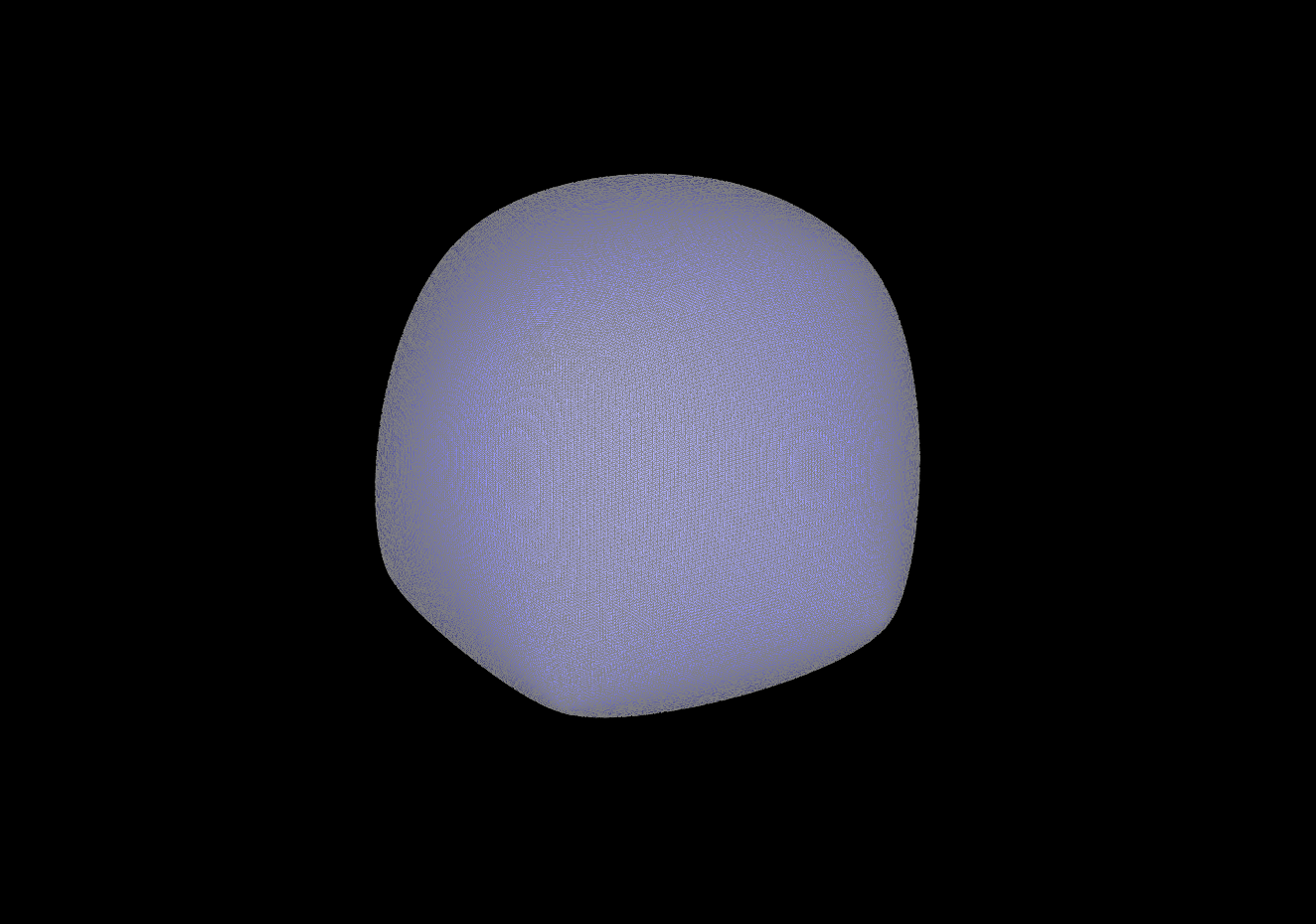
level 4 / level 5 / level 6 / level 7
By pre-splitting edges, we are able to reduce the sharp corners and maintain the shape of the original image. As we can see below, presplitting only one face keeps the flatness preserved while increasing subdivisions. This preprocessing helps because it creates more edges that can be subdivided which means we make even more edges when we flip, essentially adding more detail at each level.
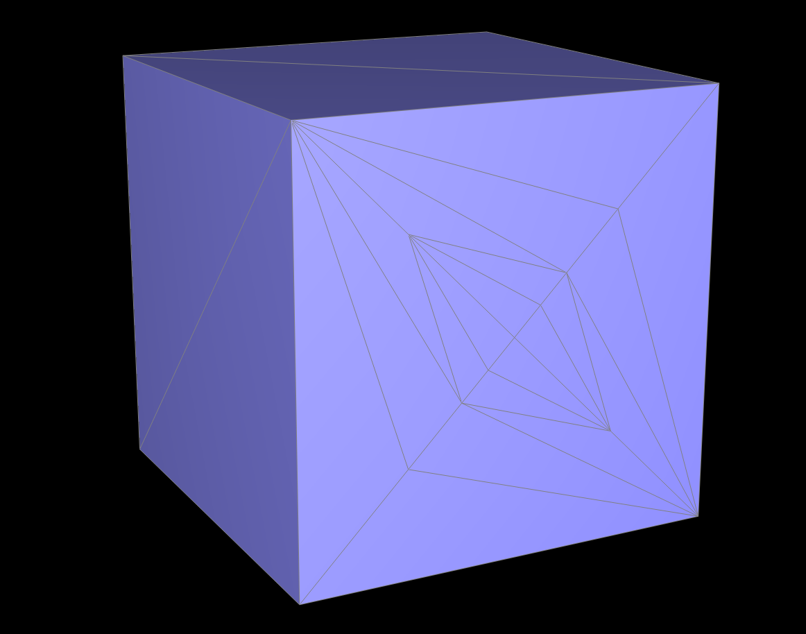
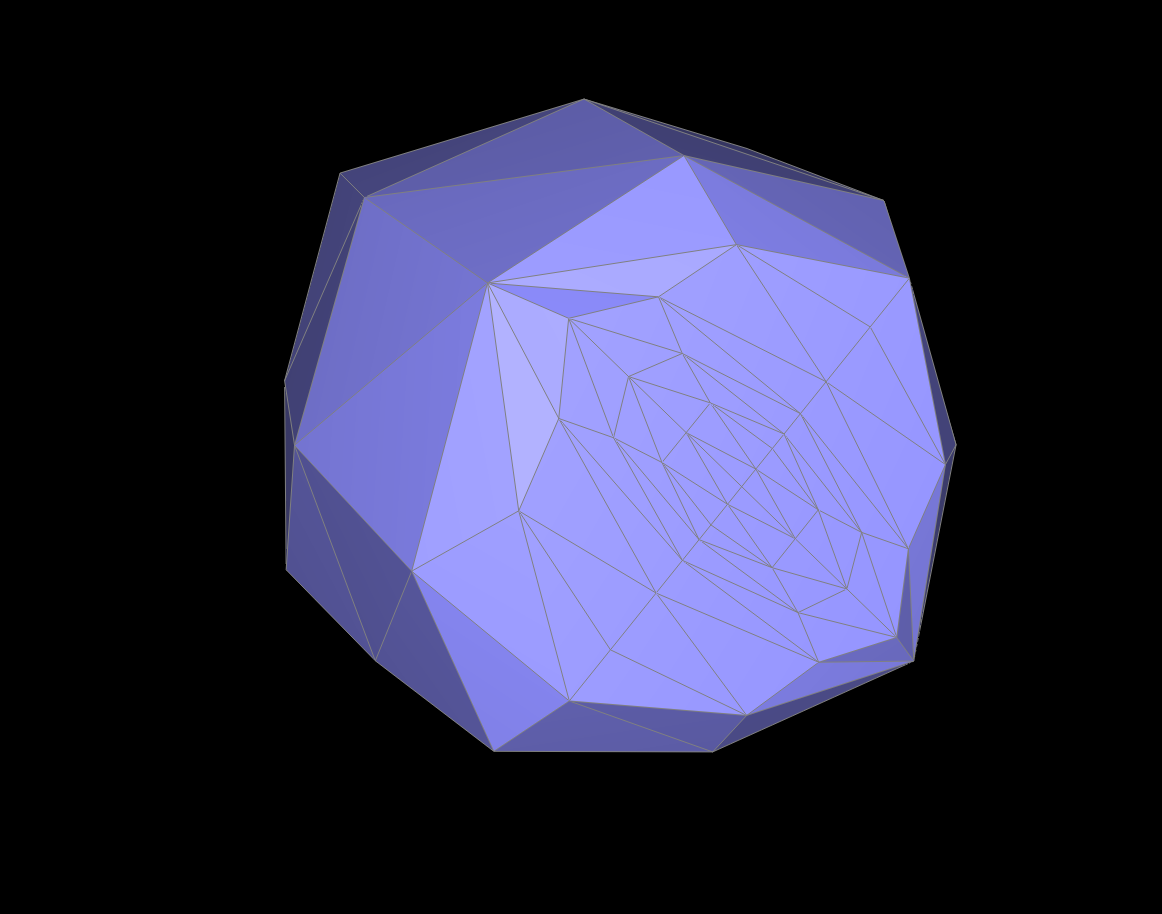
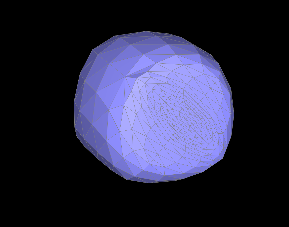
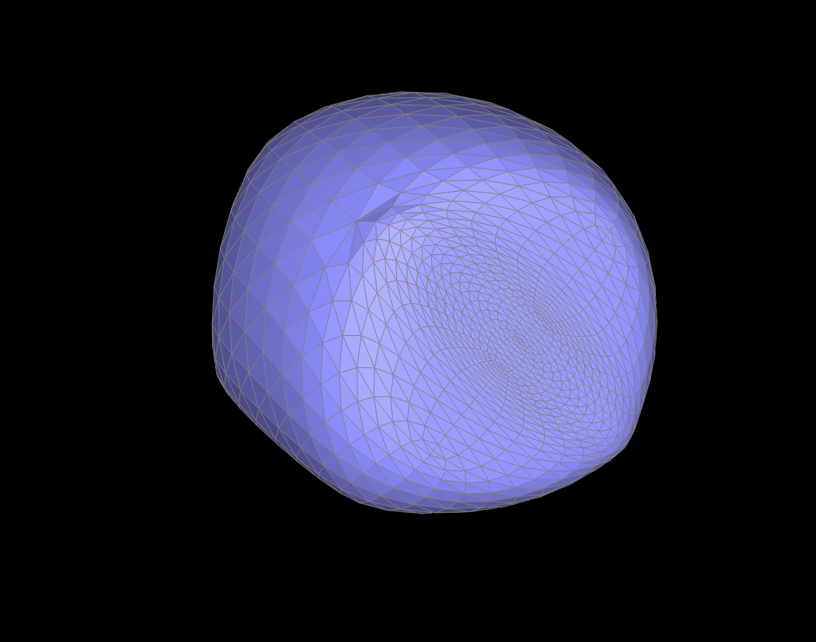
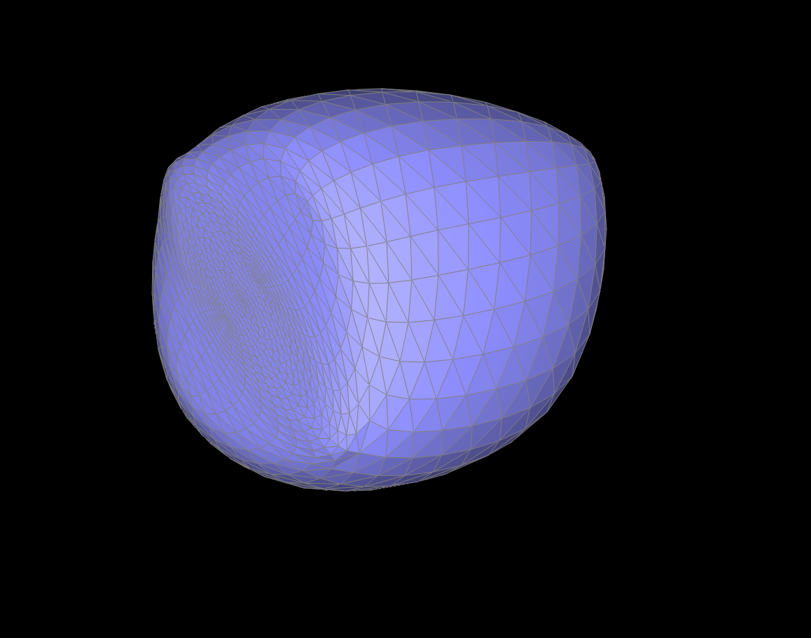
presplit / level 1 / level 2 / level 3 / yam 🍠
The usefulness of loop subdivision can be seen on the teapot and the cow which achieves a less geometric look and reduces sharp corners using these operations.
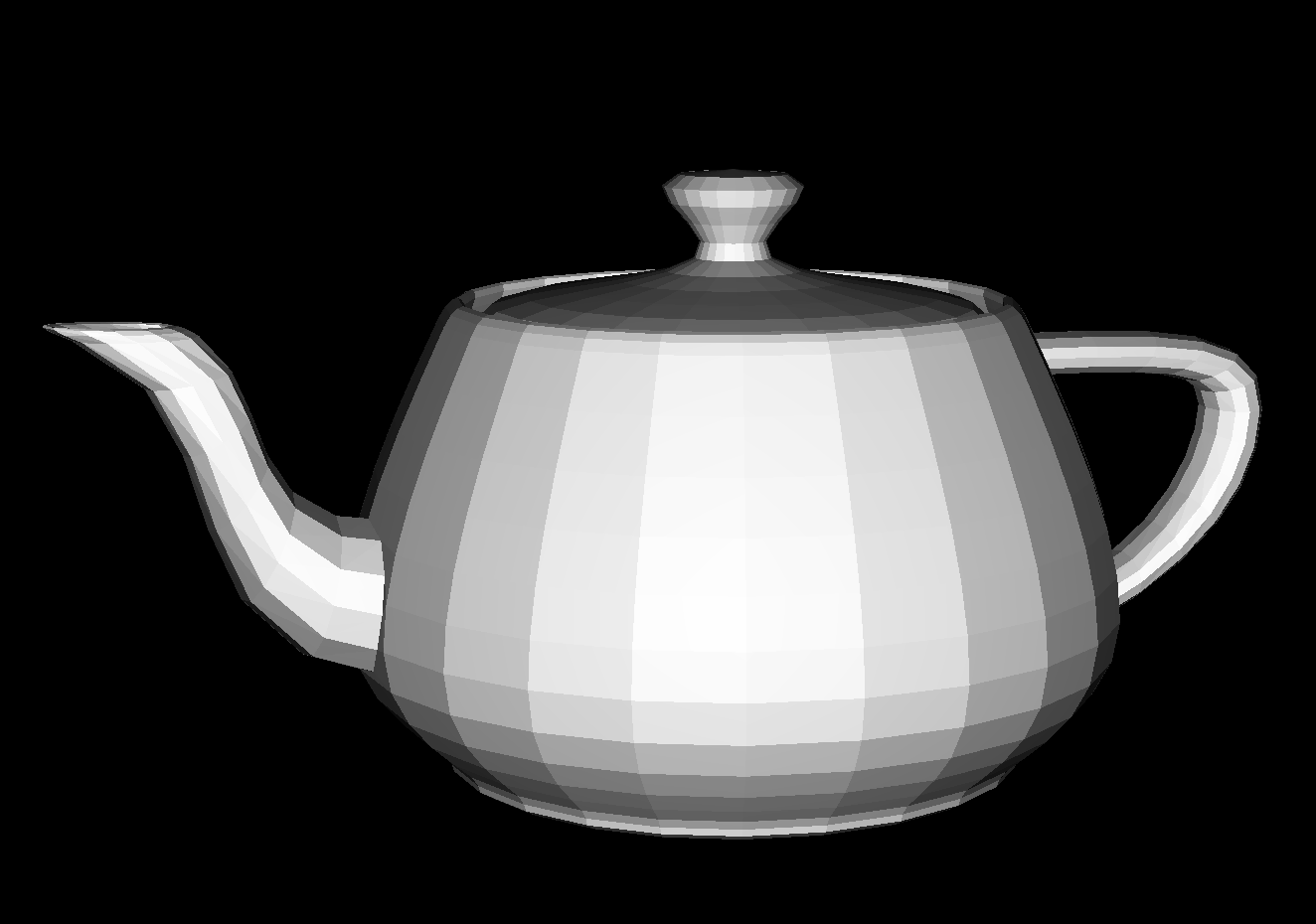
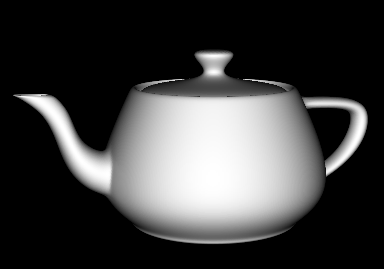
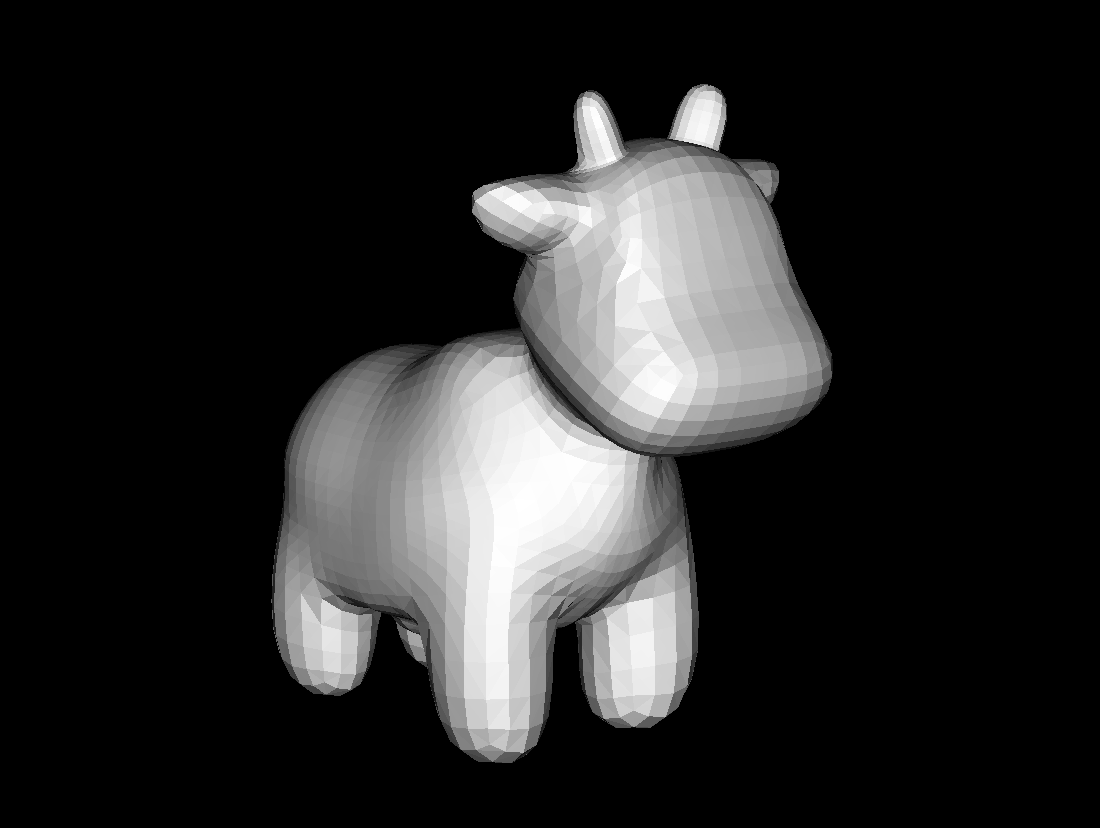
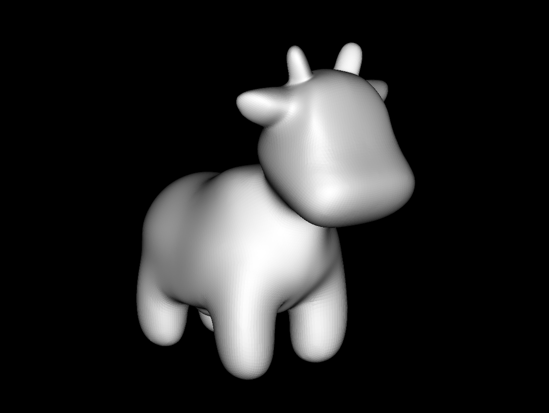
teapot before / teapot after / cow before / cow after
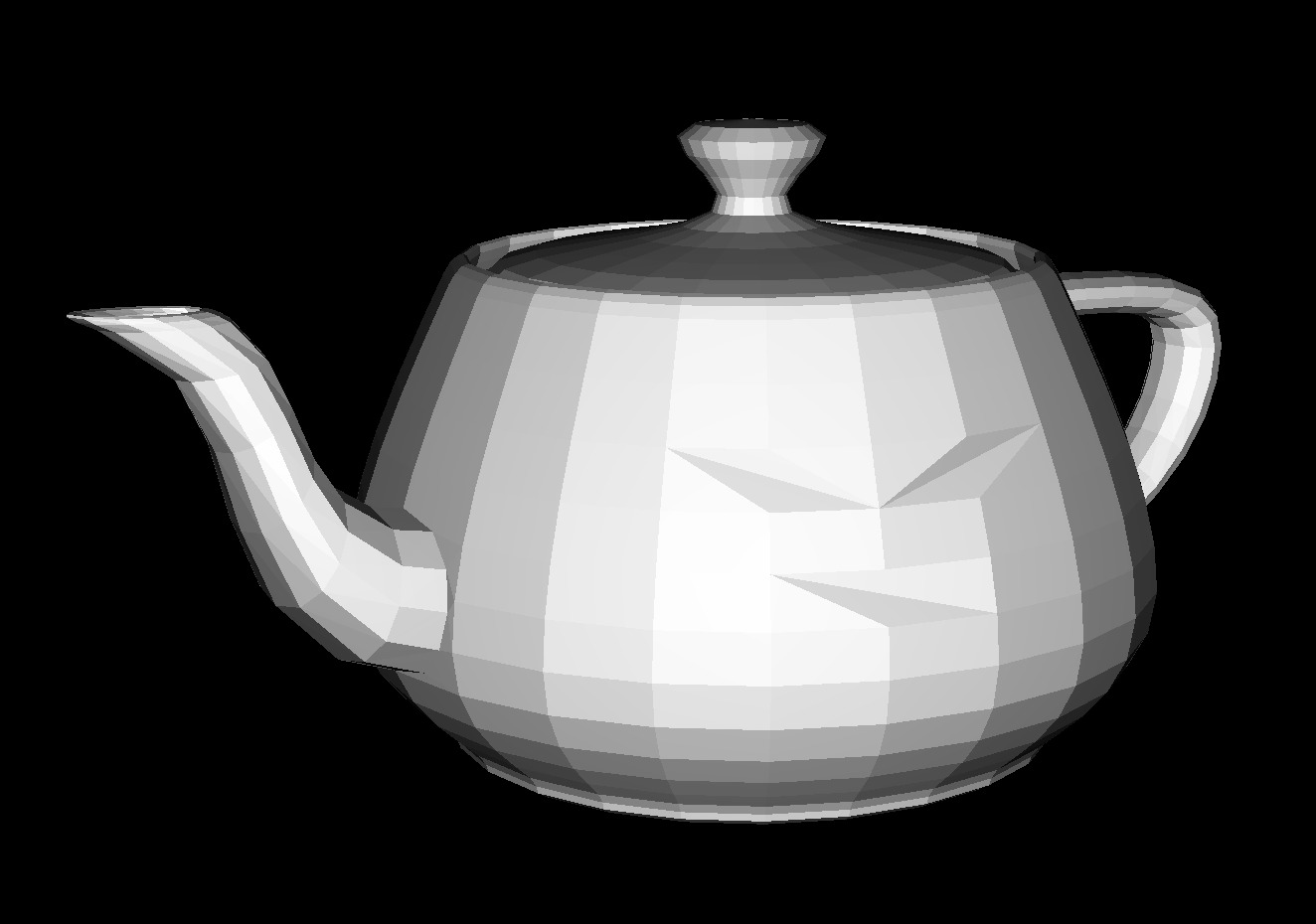
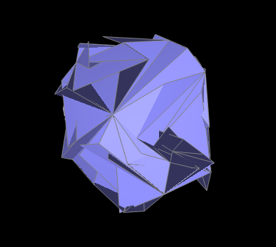
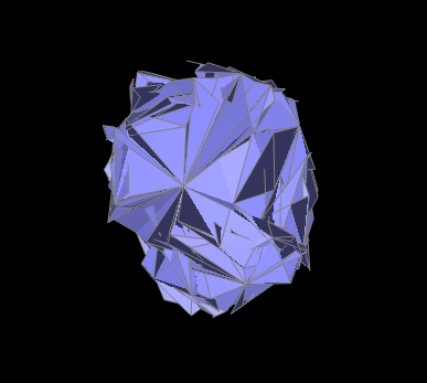
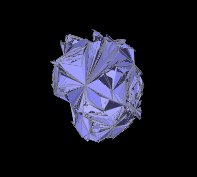
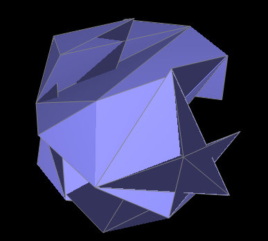
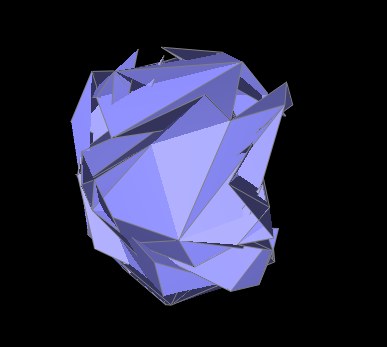
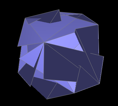
Coding up loop subdivision took a bit longer than the other parts due to some pointer bugs and keeping track of which halfedges were new, which led to some crumpled meshes during the debugging:
In this homework, I learnt about how to generate and represent rays and intersect them with triangles and spheres. After this, I worked on implementing bounding volume hierarchy. After this, was direct and global illumination where I was directly able to see and implement different bounce setups. I also enjoyed working on Russian Roulette sampling and adaptive sampling because it made the concepts we learnt much better. I faced a few bugs with the first few tasks in speeding up computation but I found that I was able to resolve them with a bit of debugging. Overall, I thought that this was a really interesting homework because I was able to implement many of the algorithms that we had only learnt about in class.
The ray generation algorithm implemented allow us to transform coordinates of an image from (x, y) to be coordinates for a Ray in the world space. In order to this, I first converted the (x, y) coordinates to be in the domain [-1, 1] instead of [0, 1]. I then accounted for the field of view calculations, taking into account the fact that hFov and vFov were in radians, not degrees. Finally, I used the c2w matrix to calculate the position of the virtual axis-aligned sensor with respect to our new coordinates. I calculated the normalized version of this vector and then returned the Ray that started from the given pos vector to this newly calculated world space vector.
To generate pixel samples, for each sample, I picked a random sample by calling gridSampler-{'>'}get_sample(). I then call generateRay on the sampled coordinates, making sure to normalize by the width and the height of the image. For each ray generated in the loop, I call est_radiance_global_illumination and sum up the total illumination from all the rays. I then take the average based on the number of samples and return a final call to update_pixel to render this pixel with the color.
In order to calculate ray-triangle intersection, I followed the Möller-Trumbore intersection algorithm. In order to use this algorithm, I first calculated a set of variables to make the calculations easier, specifically: E1, E2, S, S1, and S2. I then calculated the inverse determinant and multiplied this by the matrix: \([S2 \cdot E2, S1 \cdot S, S2 \cdot D]^T\). This gave me the final matrix, \([t, b1, b2]^T\). After getting the values for t, b1, and b2, I tested all of them to make sure that they were within (0, 1). I repeated this same calculation for the intersect function, but also added updates to the isect variable, by calculating a normal vector based on our values for b1, b2, and 1 - b1 - b2.
In order to calculate ray-sphere intersection, I followed the description from the slides and generated a quadratic equation for the intersection of the ray and the sphere. In order to simplify the calculations, I returned false if the determinant was less than zero because we want only positive roots. I then followed the same steps as ray-triangle intersection to assign values to our intersection. I also made sure to update the max clipping frame with t.
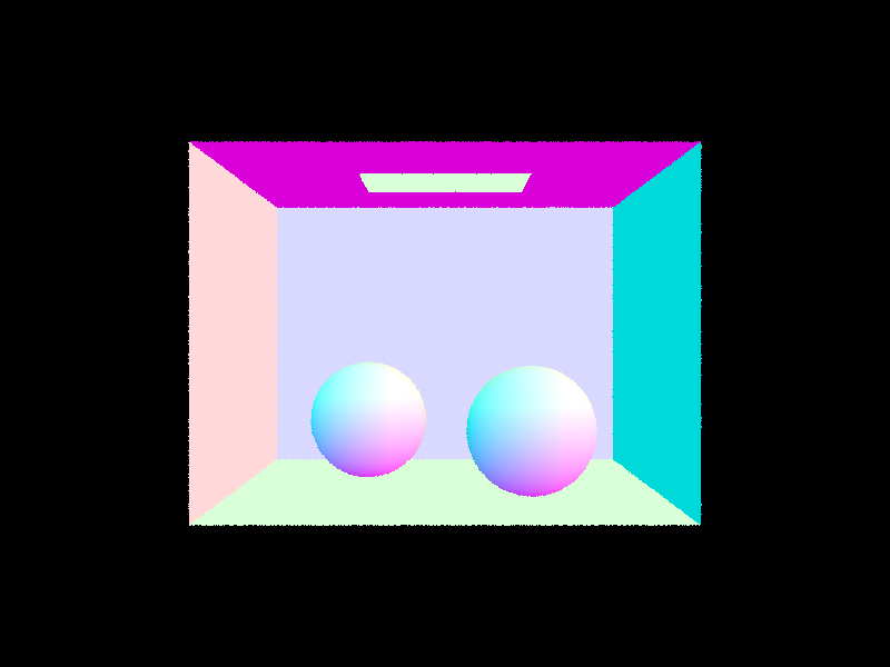
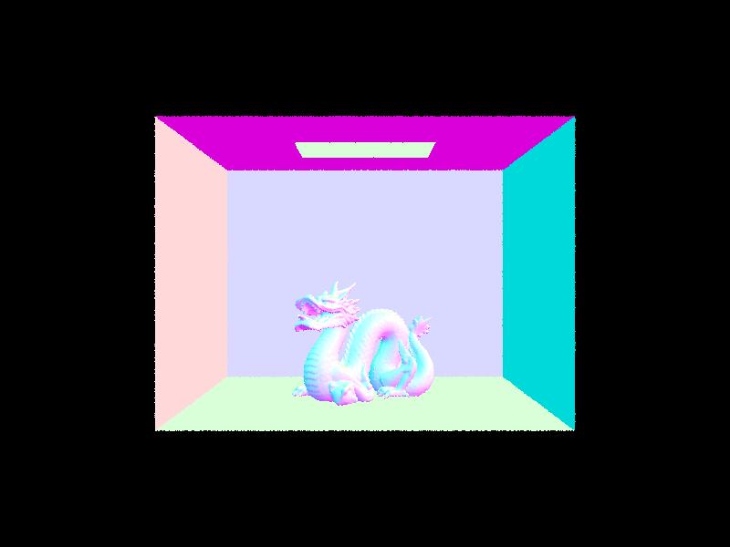
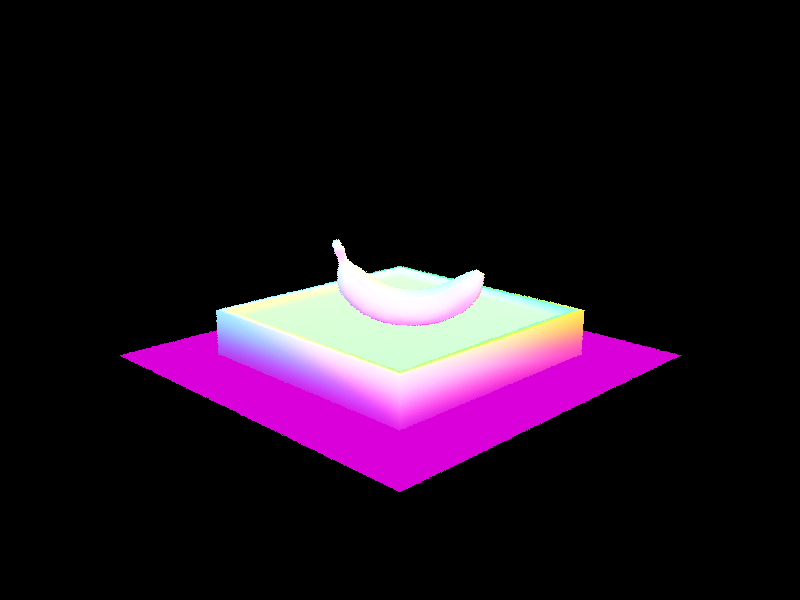
ray-sphere intersection / dragon normal shading / banana normal shading